How Local Supply Chains Influence Scope 3 Emissions (and when “buy local” backfires)

Buying local doesn’t automatically reduce Scope 3 emissions. Local sourcing often lowers emissions when it reduces air freight, damage/waste, or enables circular flows, but it can increase emissions if local production is more carbon-intensive than your current supplier. The most defensible approach is to compare scenarios using supplier production data plus logistics activity data aligned to the GHG Protocol Scope 3 Standard.

Key takeaways

Transport mode often matters more than distance for Scope 3 transport emissions.
Localisation can reduce Scope 3 Category 4 and 9 (transport & distribution), but increase Category 1 (purchased goods & services) if production is higher-carbon.
Air freight is often the biggest “emissions swing factor.”
The most defensible answer comes from scenario modelling using supplier + logistics data aligned to the GHG Protocol Scope 3 Standard.

Does buying local reduce Scope 3 emissions?

Sometimes, but only when the whole system changes in the right direction. “Local” can reduce Scope 3 when it replaces high-carbon transport (especially air freight), reduces damage and waste, and enables circular models. It can backfire when production emissions increase enough to outweigh transport savings.

Scope 3 emissions are value-chain emissions reported across 15 categories under the GHG Protocol Scope 3 Standard, and practical interpretation depends on how you define boundaries and data quality. If you need a refresher, Coral’s Scope 1, 2, and 3 explainer breaks down how value-chain emissions map to reporting categories.

A quick worked example: distance vs mode (why “local” can mislead)

This example uses the UK Government’s 2024 greenhouse gas reporting conversion factors for freight (without radiative forcing). Radiative forcing is an uplift sometimes applied to aviation to account for non-CO₂ warming effects; reporting requirements vary by standard and context.

Using those 2024 UK factors (freight, without radiative forcing):

Short-haul air freight: ~0.985 kgCO₂e per tonne-km
Container ship (example factor): ~0.0127 kgCO₂e per tonne-km

Now compare two options:

Option A (shorter distance, higher-carbon mode): 1 tonne shipped 1,000 km by short-haul air
→ 1,000 tonne-km × 0.985 = ~985 kgCO₂e

Option B (longer distance, lower-carbon mode): 1 tonne shipped 10,000 km by container ship
→ 10,000 tonne-km × 0.0127 = ~127 kgCO₂e

Same product. A longer route can be dramatically lower-emission if the mode changes. That’s before you add last-mile trucking, warehousing, packaging changes, or production differences.

Note: the UK conversion factors include multiple options for sea freight and aviation, so for published examples it’s best to link to the specific table line items used in the 2024 pack.

Why companies are nearshoring (and what it means for Scope 3)

Nearshoring/onshoring (moving production or suppliers closer to demand) is often framed as a win-win: lower emissions, more resilience, and better transparency.

There is truth in that, but only if you account for production energy mix, process efficiency, transport mode, packaging, inventory, and waste. Otherwise, localisation can shift emissions from one Scope 3 category to another without reducing the total.

When local sourcing reduces Scope 3 emissions

Local sourcing tends to reduce Scope 3 when it removes carbon-intensive transport, especially air freight, and reduces knock-on impacts like damage, spoilage, and urgent replenishment.

1) Transport & distribution (Scope 3 Categories 4 and 9)

Transport is a major source of global emissions, and the International Energy Agency’s transport overview reports that transport-sector CO₂ emissions reached nearly 8 Gt CO₂ in 2022.

Shortening supply lines can reduce emissions tied to:

Category 4: Upstream transportation & distribution
Category 9: Downstream transportation & distribution

But don’t stop at kilometres. The bigger driver is mode mix (air vs sea vs rail vs road), plus utilisation, routing, and consolidation.

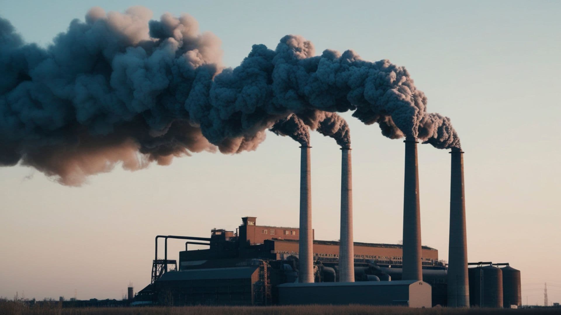
2) The air freight trap (often the biggest lever)

Air freight is extremely carbon-intensive per tonne-kilometre. In the UK Government’s 2024 conversion factors (freight flights, without radiative forcing), air freight is approximately:

Domestic: ~2.76 kgCO₂e per tonne-km
Short-haul (to/from UK): ~0.985 kgCO₂e per tonne-km
Long-haul (to/from UK): ~0.649 kgCO₂e per tonne-km

If localisation reduces reliance on last-minute air shipments (urgent replenishment, missed forecasts, long lead times), Scope 3 can drop quickly even when production volume stays the same.

When buying local increases Scope 3 emissions

Buying local can increase Scope 3 when production emissions rise enough to outweigh transport savings, especially when Category 1 changes.

1) Production emissions can dwarf transport (Category 1 is often the headline)

In many value chains, emissions embedded in the product (materials, energy, processing) are far larger than emissions from moving it.

Food is a clear illustration. An Our World in Data analysis on food emissions shows transport is ~4.8% of global food-system emissions (2015), while most emissions come from production and land-use dynamics.

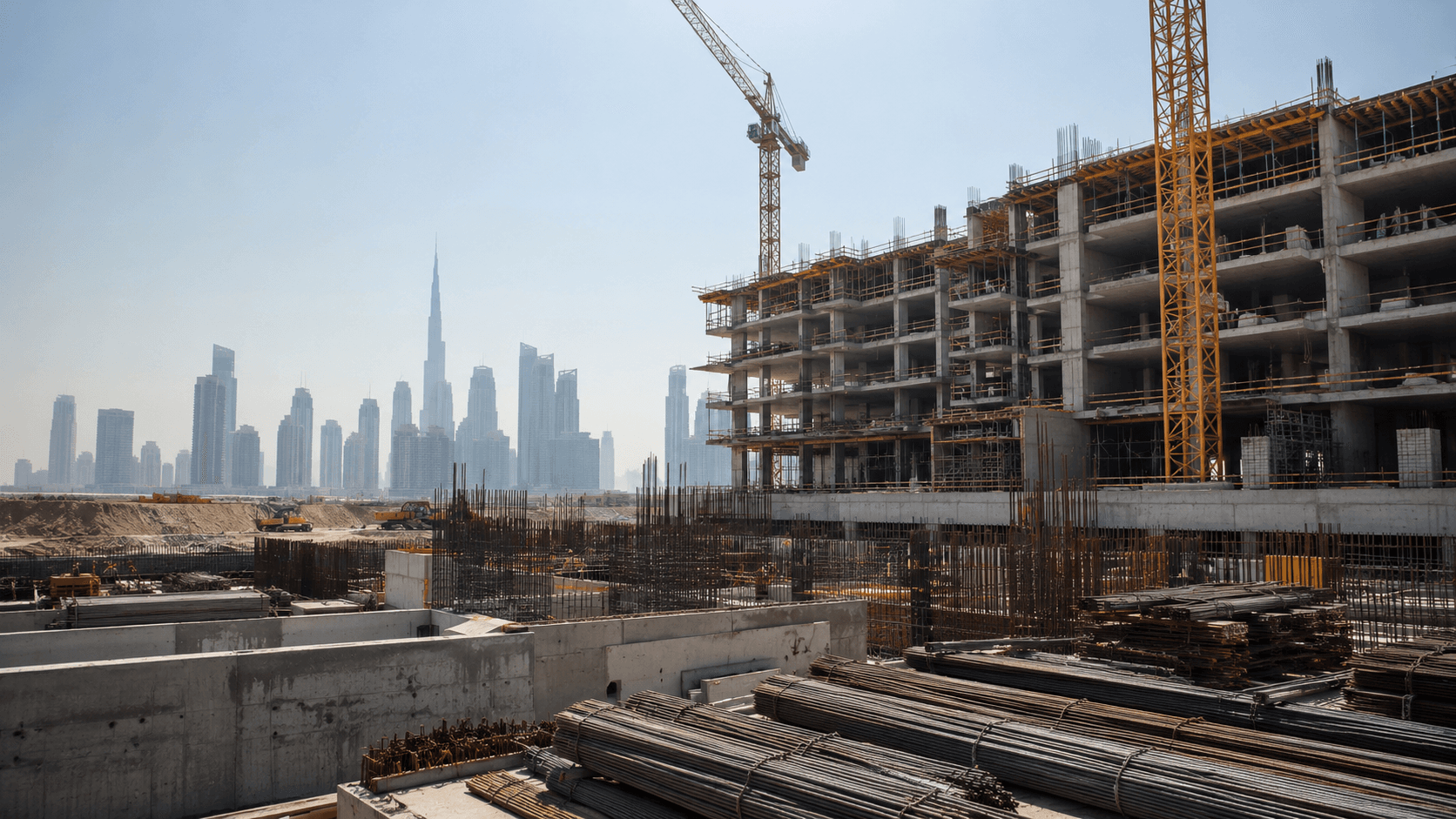
The same logic often applies to industrial products (e.g., steel, cement, chemicals): a “local” supplier can still be higher-carbon if their processes are less efficient or their energy is dirtier.

2) Supplier energy mix + process efficiency (the real “buy local” risk)

Local sourcing can change the carbon intensity of:

Electricity (grid emissions factor)
Heat and fuel
Process efficiency (equipment age, yield losses, scrap rates)

A localisation strategy that shifts procurement to a more carbon-intensive grid, or to an older/less efficient plant, can increase Category 1 enough to outweigh transport savings.

The GHG Protocol also recommends prioritising higher-quality, more specific data for the most material activities and documenting data quality and assumptions.

Indirect impacts on Scope 3: inventory, packaging, waste and returns

Shorter lead times can reduce:

safety stock and storage days
expedited shipments
spoilage/obsolescence (especially for fast-cycle or perishable sectors)

Depending on your inventory boundary and Scope 3 categories, these may reduce emissions tied to warehousing energy, waste, returns, and disposal impacts.

Packaging and damage rates

Long supply chains can require extra protective packaging, temperature control, and secondary materials. Local distribution can reduce packaging intensity, but smaller local suppliers may also have less optimised packaging and load efficiency. Either way: measure it, don’t assume it.

Circularity and reverse logistics

Local networks can make repair, refurbishment, and remanufacturing more viable because reverse logistics are shorter and more predictable, often improving both emissions and cost outcomes.

How to measure local sourcing impact on Scope 3 emissions

Treat localisation as a scenario comparison aligned to GHG Protocol methods, and use a consistent protocol baseline such as the GHG Protocol Scope 3 Standard. If you want protocol context, Coral’s guide to carbon accounting protocols covers how different standards fit together.

Step 1: Define scenarios (clearly)

Compare current state vs localised state using the same functional unit (per tonne, per unit, per $ revenue, etc.). Keep boundaries consistent between scenarios.

Step 2: Separate distance from mode

For every lane, capture:

mode split (air/road/rail/sea)
tonne-km (or activity data you can map to factors)
utilisation assumptions (load factors, backhaul, consolidation)

Define tonne-km once for clarity: “tonne-kilometre (tonne-km) = one tonne of goods transported one kilometre.”

Step 3: Don’t guess Category 1

For top suppliers/materials, prioritise:

supplier-specific emission factors (EPDs/product footprints if available)
energy mix + process data where feasible
credible secondary datasets as a fallback (documented)

Step 4: Include operational knock-ons

Model changes in:

expedited shipment frequency
inventory days and warehousing energy
spoilage/returns/damage rates
packaging weights/material changes

Step 5: Document assumptions + data quality

Write down what you assumed, why, and what data quality tier it is. This makes updates and assurance far easier.

Decision lens: when buy local reduces emissions vs backfires

Use this checklist before switching suppliers.

Localisation tends to help when:

it replaces air freight with sea/rail/optimised road
it reduces expedited shipments and improves forecast stability
it reduces damage, spoilage, and packaging intensity
it enables circular flows (repair/refurbishment/remanufacturing)

Localisation tends to backfire when:

local production sits on a higher-carbon grid
the local supplier is less efficient (older equipment, higher scrap rates)
you lose consolidation benefits and increase partial loads
emissions shift from transport to Category 1 without real net reduction

Common mistakes to avoid

Choosing “local” based on kilometres alone
Ignoring air freight and expedite behaviour
Treating spend-based estimates as decision-grade numbers for strategic moves
Not capturing supplier energy mix (which can swing the result)
Not documenting assumptions (which turns every update into a debate)

What this means in practice

Local supply chains can be a meaningful Scope 3 lever when they reduce high-carbon transport, avoid air freight, and enable circular models.

But localisation can backfire when it shifts procurement toward higher-carbon production. The win comes from optimising the whole system, not just shrinking the map.

One more point worth pressure-testing: a World Economic Forum analysis and related BCG work on supply chain decarbonization suggest that a push toward net-zero supply chains across major value chains could add as little as ~1–4% to end-consumer costs for many products in the medium term, when changes are well designed.

Next step

If you’re evaluating nearshoring/onshoring, the fastest way to get a defensible answer is to combine procurement + supplier + logistics activity data and map it to Scope 3 categories with a clear data-quality trail.

If you want a quick refresher on how Scope 1, 2, and 3 map to operational vs value-chain emissions, this explainer on Scope 1, 2, and 3 emissions covers the basics.

If you want to compare sourcing scenarios with an audit-ready data trail, Coral’s Emissions Management System shows how supplier + logistics data can be structured in one workflow, and you can also book a demo.

FAQ

Does buying local always reduce Scope 3 emissions?

No. Local sourcing can reduce transport emissions (especially if it cuts air freight), but it can increase total emissions if local production uses a higher-carbon grid or less efficient processes. In many value chains, production emissions can outweigh transport emissions.

Which Scope 3 categories are most affected by localisation?

Most directly, Category 4 (Upstream transportation & distribution) and Category 9 (Downstream transportation & distribution). The biggest swing can come from Category 1 (Purchased goods and services) if supplier production emissions change.

Why does transport mode matter more than distance?

Emissions per tonne-kilometre vary massively by mode. Air freight is typically far more carbon-intensive than sea or rail, so a shorter route by air can emit more than a longer route by sea.

How can we measure localisation impact credibly without perfect data?

Start with scenario comparisons using available logistics activity data (tonne-km and mode splits) and prioritise supplier-specific primary data for the most material categories. Use secondary datasets only as a fallback, and document assumptions and data quality.

What’s the quickest sanity check before switching suppliers?

Compare (1) supplier production footprint drivers (energy mix + process efficiency) and (2) the transport mode mix, especially whether air freight or frequently expedited road shipments are involved. If either changes meaningfully, localisation can materially shift your Scope 3 outcome.